Modern for exploration and analysis #
‘The modern geospatial stack’ isn’t really a helpful thing to say when trying to describe a whole field. But it mostly means ’not a typical commercial package’. At least that’s my take. It means thinking about geospatial analysis as more like a slightly specialized case of typical data science, and that means a assembling a toolkit from the array of open source and commercial tools out there.
I’ve been wanting to dip my toe in this arena for a while, and getting back to Woolpert has afforded me that opportunity. Rather than learn in isolation, I decided to poke at a small question that came up at work, namely: how can one more easily source data from the U.S. Federal Aviation Administration to understand and visualize ground-based obstruction in airspace.
Said another way: show me things that aircraft can collide with as they’re taking off, landing, or otherwise flying really low. And depending on your background, that may sound very odd, or incredibly useful.
Reproducible Experiments #
Something that I personally like about the toolkit for data science and data exploration is that it can be self-documenting and reproducible. If you can’t get the same results each time you run a deterministic set of steps, then something is not working correctly.
The exception is when either the underlying data are changing, or the algorithm is evolving. But excepting those cases, there’s something really nice about being able to read–literally from top to bottom–the exact steps that were needed to get from point A (hypothesis or generalized goal) to point B (an answer that is a reproducible). It’s like a re-runnable version of the old fashioned lab book. And it’s no mistake that ’notebook’ has become the noun-of-the-day in data science.
The tooling for this has evolved over time. My own personal journey has led me from macros inside GIS tools, to shell scripts that string together various input-output operations (like ‘convert this data’, ‘summary it using an open source library’, etc.), up to today where I’m mostly using Jupyter Notebooks.
Get started with Jupyter and load some geospatial goodies #
Jupyter used to be an exclusively Python-centric environment for documenting ’lab experiments’. Indeed, the core is still seen in the UI and documentation as IPython (interactive Python, I think?), and using Python package management tools remains a common way to get up and running. However, Jupyter now extends beyond Python.
Here’s how I typically get up and running. And you will notice that it’s all rather command-line-y and not point-and-clicky. That may turn you off but it does make things very reproducible:
| |
At this point you can open your browser to the URL indicated and start experimenting.
A basic notebook
There are two cells. One is markdown and the second is Python. You can also write system calls such as a shell command using a leading ! or various shortcuts like %cd to change directory or %ls to list files.
It’s Python (most) of the way down #
Having said that Jupyter notebooks are multi-lingual, the geospatial toolkit is overwhelmingly Python-based, with workhorse native (C, C++) libraries like GDAL and PROJ having excellent Python bindings like rasterio for GDAL.
Couple that with the fact that data science toolkits themselves are predominantly Python–with libraries like numpy and pandas leading the way–I’ve been exclusively using Python for my experimentation and learning. If you’re an R fan or MatLab devotee I’m sure there are plenty of libraries in your ecosystem too…it’s just not where I hang out because of the geo-centric nature of my work.
It’s not all roses: for those libraries that aren’t just a pip install ... you still need to know your make build... approach to software installation. I’m on a Mac most of the time so I tend to use homebrew instead, e.g., brew install spatialindex to get libspatialindex installed. But the rest of the time I’m using pip.
Not entirely Python #
The format of a notebook (*.ipynb) file is not Python, then. But it does provide an execution environment for Python. To make this clear, here are the first lines of the notebook I’ll write for this post:
| |
It’s a mixture of content types saved in what looks like a JSON format; for example, look at the presentational decorations like the "\n" for new lines.
I strongly recommend just using the browser-based editor or something like the Visual Studio Code Python extension by Microsoft that provides a nice integrated experience (I use both). But it’s good to know that there’s no magic here. Just text.
Getting something done #
Back to the matter at hand. I want to:
- Download some data from a government website (FAA).
- Take a look at it so I understand the structure.
- Geo-enable it so that I can see the spatial distribution.
- Export the data into a common geospatial format.
- View it in a web page.
To do that I’ll write a Jupyter Notebook to access, validate, and export the data. Then I’ll switch to a webpage for a snazzier visualization.
Using Geopandas #
First up, I installed geopandas. This is the geo-aware extension to the ubiquitous and amazing pandas library. If there’s a multi-tool or Swiss Army knife of data analysis in Python, it’s pandas (which itself builds on numpy and others). Or maybe pandas is the big blade in the pocket knife? The point is, it’s sharp and versatile.
Geopandas extends the data types, predicates, visualization with map stuff. Let’s take a look at the very first code cell:
| |
Wait…what’s that weird !{ } surrounding the sys.executable call?
You can indeed use pip to install your dependencies for a notebook. In this case I would have done pip install geopandas. However, following some great advice for more portable notebooks that don’t accidentally dump a ton of conflicting dependencies in your system Python or even a virtual environment, you can use the magic ! notebook function to ‘call pip in the context of the current Python environment and install geopandas’. So yes, you should use pip and virtualenv as well, but this ensures that the slightly confusing Jupyter kernel (i.e., Python runtime) is not side-stepping your careful environment setup.
That might seem like a small thing but I spend a lot of time trying to debug some missing dependencies on my system.
If that seems a bit tricky, just make sure you’re always operating in a virtual environment and use pip freeze -r requirements.txt or similar to keep your dependencies tight and understood.
Back to geopandas. Now that it’s installed you can do some geospatial magic. First let’s get that data.
Executing shell commands #
To get the data from the FAA website I want to run a couple of shell commands. Rather than jump out of my notebook and run them manually, I want to document precisely and forever where I got the data from. Using the ! magic function helps again. Take a look at how this is accomplished in a notebook cell:
| |
It’s just three basic shell commands to remove any existing files, download fresh data, then uncompress for further processing. There’s absolutely nothing special here other than the leading !. Using environment variables works as expected (%env) but I don’t need them here. Simple.
One of the best parts about Jupyter notebooks is that the results are saved inline. Not only do you get to see the output from the execution of each cell (md -> html, python -> console, etc.), but that it’s stored inline in the notebook file. So it’s possible–and really helpful–to run File > Download as… > HTML in your Jupyter browser UI and have a complete record of your analysis. Just like a lab notebook! Here’s what the previous cell outputs:
| |
It’s just the STDOUT from my shell. Neat!
Import and preview data #
Finally, we get to use geopandas. Using the read_csv function pulls the CSV file into a native pandas Dataframe structure. Then the shape function prints a bit of basic information about the data.
Not using an encoding has worked for me in the past. But not this time! Following a tip about dealing with data that was exported from Excel, the use of cp1252 seems to fix things.
| |
Pandas has a ton of useful features just at this stage, but the shape function gives me an idea of the size of the data:
| |
Whoa! Almost half a million obstructions are being tracked by the FAA, and each with 19 attributes. That could take a while to work with…
Being a geographer, I really want to see the spatial distribution. Geopandas can read coordinates from columns in a regular pandas dataframe and create a ‘geometry’ column suitable for analysis and visualization.
If you’re not familiar with map projections and coordinate reference systems (CRSs) then the gdr.crs will look a little weird. Not to worry: it’s just how we tell geopandas that this is latitude and longitude data and that we want to use a ‘worldwide web mercator’ projection. It means that the data will be compatible with lots of online mapping tools. More of that in a minute.
| |
And after a few seconds, geopandas has done its magic on all 480K+ records:
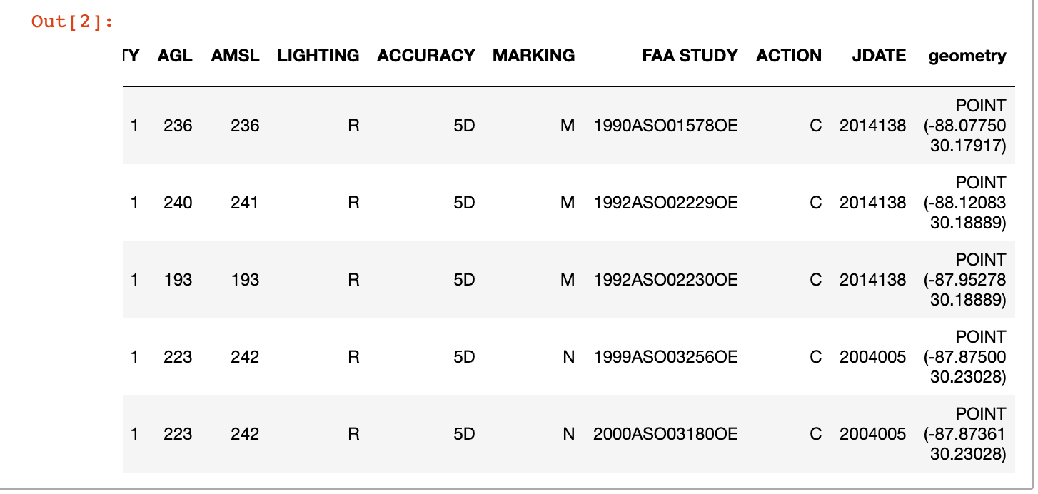
The head operation shows a new geometry column
Nice!
Preview on a map #
The table view is nice, but like I said: I want a map. Geopandas depends on a ton of other native and Python libraries to work its magic, including matplotlib, shapely, and descartes. Here’s what it takes to render a map:
| |
I skipped a couple of steps that you can find in the source notebook around getting some background data (country boundaries), but it’s pretty simple to generate a map:
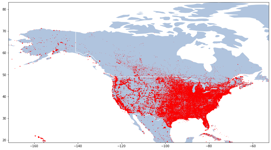
Simple dot map showing the distribution of FAA-monitored obstructions
I’m not going to lie; that took a while to render on my MacBook Air (~15-20 seconds). But remember that I can just export the result as HTML, and that the *.ipynb file embeds the encoded image so that I don’t have to run the expensive function just to the see the map. It’s already baked in (look at the source notebook and you’ll see that text-encoded image).
Export for further use #
The last step in my notebook is to export the data into a useful geospatial data format. CSVs are nice and transportable but they don’t immediately lend themselves to further use by many geo libraries.
There are lots of options but I’m going with the massively verbose but lingua franca GeoJSON format. It’s JSON…with geo!
| |
The full ~500K records are dumped into a 230MB text file called dof.geojson. But because that takes so darn long to open, I also used the pandas query function to filter down the massive dataset into something more manageable: the obstructions in the State of Minnesota. Here’s one feature courtesy of cat mn.geojson | jq '.features[0]':
| |
And that took a really long time to export (2 minutes? I think?!). If I was serious about performance I would have sliced off the attributes I don’t need, etc. But I’m experimenting so it’s OK. No need to optimize when I’m just poking at the data in an exploratory fashion.
Map using deck.gl #
I’ve been wanted to dink around with Uber’s deck.gl geospatial visualization library for some time. Mostly in the context of recent work on 3DTiles and their loaders.gl work with the folks at Cesium. But for now I’ll set my sights lower and just try to get an interesting visualization of my GeoJSON obstruction data. At this point, I’m out of Jupyter and writing a simple HTML document.
If you want to follow along, crack open a terminal and start a little web server thus: cd the-right-folder; python -m http.server. First, the output in the browser:
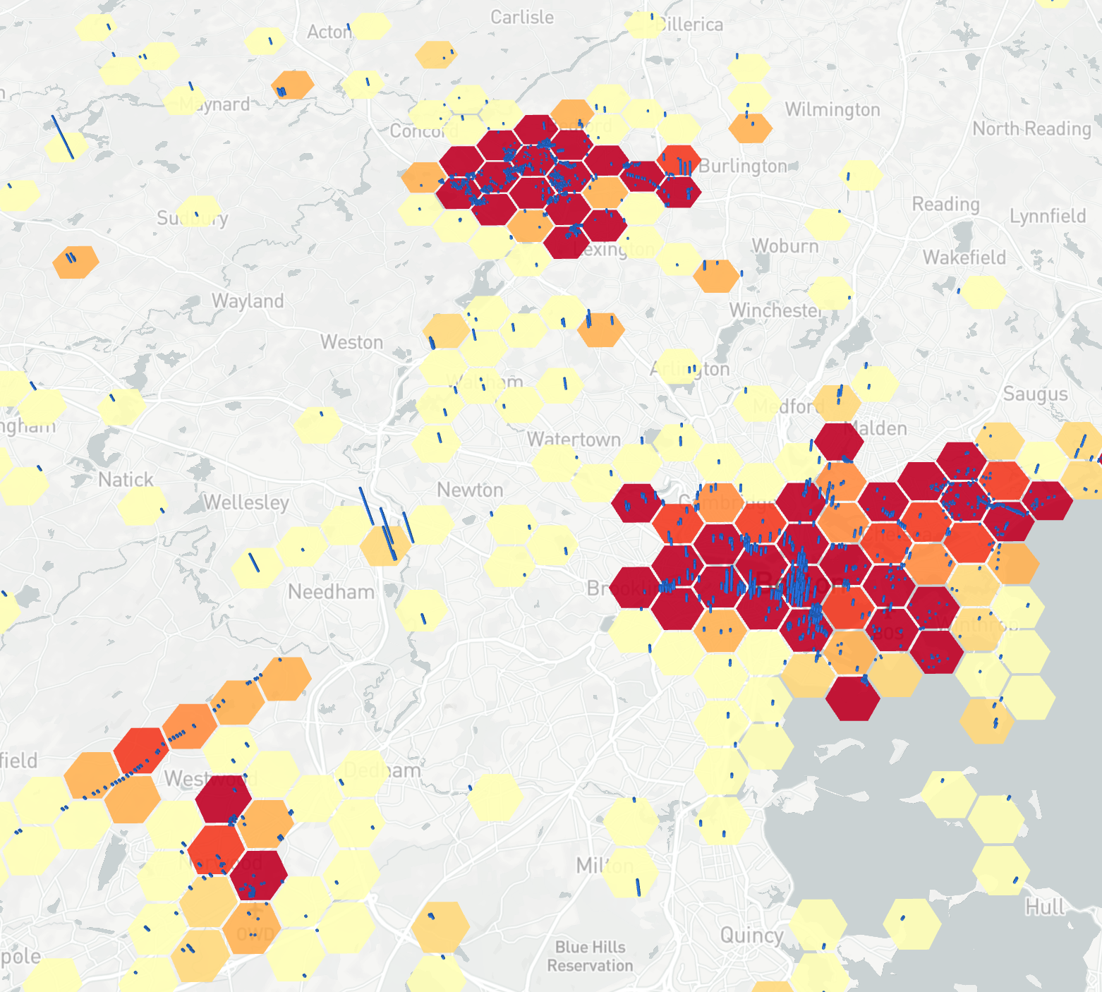
deck.gl map showing a HexagonLayer aggregating the obstruction in 1km cells, and a ColumnLayer extruded by the elevation above ground level
And the code, borrowing liberally from some great deck.gl samples:
| |
The interesting parts are in the definition of the HexagonLayer (line 45). The dataTransform: data => {return data.features} (48) took a while to figure out. GeoJSON wraps the individual features in an outer collection container in an array called features. So post-load, the dataTransform method gives a one-time filter to shape the data that the HexagonLayer will consume. Having done that, the mapping provided by getPosition: f => f.geometry.coordinates operates on a per-array element basis to tell HexagonLayer which fields contain the location data. You can see the same pattern repeated in ColumnLayer (63).
Apart from that it’s a fairly unexciting ripoff of one of the deck.gl examples. If you want to reproduce it, don’t forget to generate your own MapBox key (71).
In the spirit of experimentation, it is extremely slow and non-optimized. Yes, loading the same 240MB GeoJSON file twice (!) in the same page is very, very undesirable. But hey, it works on my machine and I can experiment. Actually, you can see on lines 42-43 where I was using the small Minnesota dataset. In a real application we’d be doing this aggregation work on the server, and probably using an optimized web delivery format like 3DTiles or MapBox’s own MBX format…or throwing it all in PostGIS and letting it handle that natively.
Summary #
My general thoughts:
- The rapidly maturing open source geospatial data science toolkit build on a rich set of tools, practices, and libraries from the data science community.
- Python seems to have the geospatial mindshare.
- It’s all just source code. With typical good practices for Python projects–and source code in general–we have a repeatable, predictable model.
- The stitching together is familiar to anyone with an open source or POSIX-based mindset. It’s not all in one package, but then again ‘data science’ is 90% finding data and methods, and 10% stitching it together to derive insights (that 90% part probably speaks to my workflow rather than some universal truth!).
Good luck geo-spelunking with this interesting and diverse toolset.