August 18, 2021
regex google sheets
Using some little Google Sheets tricks for an agenda
If you just need a template make a copy of the source spreadsheet and follow the instructions.
One of the things I find myself doing occasionally is putting together workshops, team meetings, and the like. That typically involves creating an agenda, and I usually reach for Google Sheets to create that. Columns for Start Time, End Time, Session title, session lead, etc. And during that agenda creation process there’s often some churn: move this meeting, change the length of that one, switch to a different day, and so on.
This is really obvious stuff but there are a couple of tips I’ve learned…and keep forgetting…so I’m writing them down here.
The two things are: (a) how to highlight non-meeting rows like breaks, and (b) how to make quick changes to the order or duration of sessions a lot easier.
Highlight the rows with food or coffee
I want to highlight the entire row of the agenda where there is a break or lunch. There are a few ways to accomplish that, but I want Google Sheets to do more of the work. So how do you:
- Find a cell containing either the word ’lunch’ or the word ‘break’,
- ignoring the case so that ‘Lunch’ is just as valid as ’lunch’,
- then conditionally highlight all the other cells in the row containing that match?
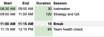
See how the row for the Break is gray across the board whereas the other session titles are not filled? That’s the goal.
Highlighting agenda items with food or coffee
Highlight a row
Highlighting the row is something I’ve done multiple times but always forget how to do.
Guess I should write it down?!
Anyway, I found a detailed and effective tutorial showing how to use Format > Conditional formatting with a Custom formula to get the job done.
I tend to select the entire set of columns I need rather than a rectangular range of cells (A:F for example, vs A1:F10000).
But really that’s not the point.
But what should the custom formula say? Maybe a couple of SEARCH functions with an OR in there to cover both ’lunch’ and ‘break’?
And remember that we want LOWER case too.
Like so: OR(SEARCH("lunch",LOWER(D14),1),SEARCH("break",LOWER(D14),1)).
That would work…except it doesn’t.
The first case of a non-matching result throws a #VALUE error, so not finding ’lunch’ would prevent me SEARCH-ing for ‘breakfast’.
In essence, this only works when the first string is found:
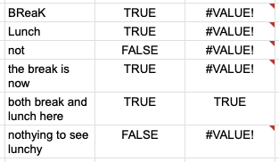
Lunch or some breaks are not an option
Fiddling with XOR and friends didn’t help either.
On top of that, I also wanted to add ‘dinner’ and not the word ‘breaking’ (like a session called ‘Breaking the build’ is not about food!).
So I looked instead at my old nemesis friend regular expressions.
Regex to the rescue
The REGEXMATCH function in Google Sheets is the one I wanted.
It takes two arguments: the text (or cell containing text) to search for, and a regular expression following the Google RE2 syntax
I quickly came up with (break\b)|(lunch\b) to match whole words, but I couldn’t immediately figure out the case-insensitivity.
Google RE2 does indeed support the case-insensitive i syntax, so I tried adding /i to the end of the expression.
That didn’t work but a little Googling turned up a great tip on how to set the case insensitive flag in Google Sheets
Adjusting this I have a regular expression REGEXMATCH(D14,"(?i)(break\b)|(lunch\b)").
The (?i) section is the place where any global setting is applied, in this case the i meaning ‘ignore case’.
And even with the LOWER() expression removed I still get the result I’m looking for:
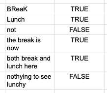
Case insensitive results again
Back to highlighting the whole row!
I know that the work ‘break’ or ’lunch’ (or ‘dinner’!) would always appear in column D so I need to anchor on that one.
As a result my Custom formula on the Conditional formatting panel looks like this: =REGEXMATCH(($D1),"(?i)(break\b)|(lunch\b)|(dinner\b)") = TRUE.
Note that I’m including the leading = sign, and the LOWER is now gone in favor of the (?i).
With that in place, any cell D-something containing ’lunch’ or ‘break’ (but not ‘breakfast’ or ’lunchy’) will have a nice highlight.
Automatically determine start and end times for sessions
One thing that always bugs me about putting an agenda together is getting the start and end times correct. You start with columns for Start and End time. Then you add a few rows with new sessions. Then someone says “Why don’t we make the second session longer?”, or heaven forbid: “Let’s move that session to later in the day”. Aaaargh! Now I’ve got to fix my start and end times.
I know what you’re thinking: why don’t you just have the Start Time of the next session point to the End Time of the previous session? Genius!
Except in practice I find a more common need is to change the length (Duration) of a session rather than shift it around. And for that I typically find find it easier to change the length (Duration) in minutes rather than do simple but (for me) error-prone clock math.
And even if that weren’t the case, dragging rows around to switch sessions is a problem because Google Sheets magically (and annoyingly in this particular case) remembers which End Time cell you session was pointing to. Instead, we want each agenda item row to always point back to the row just before it and stop doing magic.
INDIRECT and ADDRESS for less magic
Enter INDIRECT.
This is a function that lets you define a relative reference to a cell rather than an alphanumeric or explicit reference to a cell.
Or to quote a great blog post:
The
INDIRECTfunction in Google Sheets takes in the cell address in the form of text and returns a cell reference. It works in the opposite way to theADDRESSfunction, which returns an address in text format. source
That’s really handy in our case, especially if we harness the power of COLUMN and ROW.
Consider the following agenda where I want the start time for the Strategy and QA session to always start after the End time of the preceding session, which in this case is the Icebreaker session.
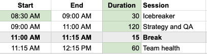
Reference pointers
The value of the Start cell for the Strategy and QA session contains the following: INDIRECT(ADDRESS(ROW()-1, COLUMN()+1)).
Illustrative example
To decompose what’s going on here, we can look at the following:
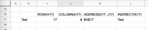
Elements of the formula
We want to use the value of the field H17 in cell L17 but–critically–we DO NOT want cell L17 to simply say =H17.
As a reminder, that’s because if we copy and paste the cell L17 somewhere else on the sheet it’ll still point right back to H17, which is NOT what we want.
Instead we want to always point to the field that is “five columns to the left”.
Real example
Back to our real example then: INDIRECT(ADDRESS(ROW()-1, COLUMN()+1)) in the cell A6.
Here we’re just doing a little extra calculation to get a relative row and column:
- Get me the current row number (6), then subtract 1 to get the row just before me. That’s row 5.
- Get the current column number (1 or the
Acolumn) and add 1 to get the 2nd orBcolumn. - Get me the alphanumeric address of the column/row at
5,2. That’sB5. - Use the alphanumeric value to indirectly get the value of cell
B5, which is the End Time of whatever session precedes me.
This may seem like a ton of work to get a value. But trust me, it makes for much more resilient copying and pasting of cell values, dragging and dropping of rows, and tweaking of session durations.
A worked example
Feel free to copy the demonstration sheet.